This project asked a specific question: which chemical measurement was most useful for identifying recent cannabis use? Finding a chemical in a sample was only part of the answer. We also needed to know when the sample was taken and how much of the chemical counted as a positive result.
I worked on a three-person student analysis using R. My work covered preparing the data, comparing measurements, and interpreting the results. We studied blood, saliva—called “oral fluid” in the dataset—and breath. The chemicals we measured are called biomarkers: measurable signs of exposure.
Make the comparisons fair
The dataset included placebo, lower-dose, and higher-dose groups, with measurements before and after cannabis use. A placebo group provides a comparison without the active treatment. The records also distinguished frequent from occasional users, since their starting measurements could differ.
I standardized column names and group labels, assigned observations to time windows, and removed duplicate observations within those windows. The first 0–30 minutes had the most data, so that became our main comparison. We also examined blood samples from 31–70 minutes.
We first looked for measurements that could separate the groups at all. Some chemicals were zero across the treatment groups; others were already present in placebo samples. Neither pattern offered a straightforward signal of recent use. Breath had only THC measurements, which limited the comparisons we could make with it.
What counts as a positive result?
A test needs a cutoff: the concentration at which it calls a sample positive. A lower cutoff catches smaller amounts, but can also flag more samples that should count as negative. A higher cutoff can miss cases we want to identify.
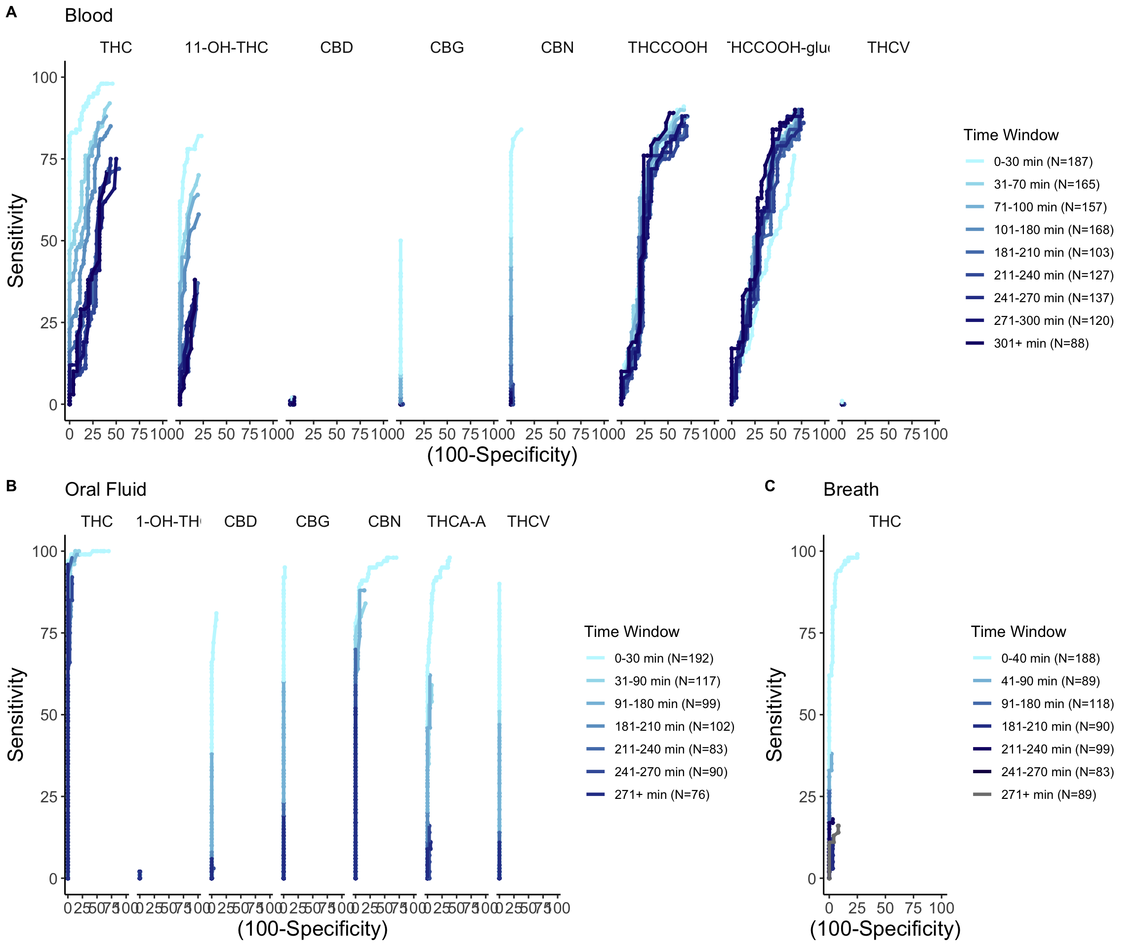
We compared that tradeoff using ROC curves. The vertical axis shows how often a test catches the positive cases, called sensitivity. The horizontal axis shows how often it incorrectly flags negative cases. A curve toward the upper-left corner catches more positives with fewer false alarms. Specificity is the share of negative cases the test correctly leaves unflagged.
Read these curves toward the upper left: higher detection, fewer false alarms. The early time windows gave the strongest results in this analysis.
Why we settled on saliva and THC
THC in saliva during the first 0–30 minutes was our preferred combination. Blood offered more samples and chemicals, but the saliva measurements were closer between frequent and occasional users. Within this dataset, that made a shared cutoff more plausible.
We compared cutoffs of 0.5, 1, 2, 5, and 10 ng/mL. This unit means nanograms of a chemical per milliliter of sample. Our analysis favored 2 ng/mL: the higher cutoffs missed too many positive cases, while the lower ones carried more false-positive risk. In the later 31–70 minute blood comparison, THC also performed best among the candidates we examined.
The code below applies the same set of cutoffs to each time window in the saliva data. That made it possible to compare how each cutoff performed as more time passed, rather than choosing one from a single measurement.
Reading the code. The function pairs each window’s start, end, and label. pmap_dfr passes those windows to sens_spec one at a time and combines the results into a table. The call below it selects THC in saliva (OF) and the five cutoffs discussed above. Source: cs01.html, sens_spec_cpd() and the THC cutoff comparison; line breaks adjusted. The supporting functions and prepared data are defined elsewhere in the original analysis.
Two chemicals can move together without being equally useful
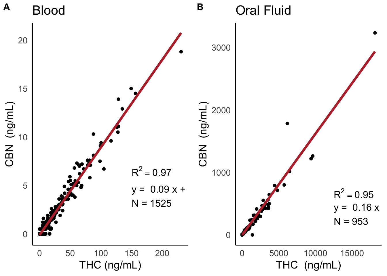
We also compared THC with CBN, another cannabis-related chemical. The scatter plots show that samples with more THC often had more CBN. Each dot represents a measurement pair; the line summarizes their relationship.
That relationship did not tell us which chemical made the better test. For that decision, we still needed the cutoff comparisons and the ability to distinguish positive from negative cases. A close relationship between two measurements is different from a reliable decision rule.
THC and CBN tended to increase together. This helped describe the data, but did not replace the test-performance comparison.
What the result means
The project’s conclusion was a particular sample, chemical, time window, and cutoff—not a claim that any positive cannabis test establishes recent use. Stating those conditions is part of making the result understandable.
The 2 ng/mL finding belongs to this dataset and analysis. It is not a legal limit, a measure of driving impairment, or a medically validated test. We compared existing measurements; we did not evaluate a deployed screening system.